Hello, welcome to todays blog which I am going to go through my attmept at sliced. If you never hear of sliced its competitive data science which you have 2 hours to create a machine learning model. Catch the show here on tuesdays late a night for us Europeans

https://www.twitch.tv/nickwan_datasci

One of the recent rounds used data on new York Airbnb so I took the dataset without watching the whole show. Set a stop clock with 2 hours on it and away I went.

0 Mins

library(tidyverse)


library(tidymodels)

setwd("~/Projects/Sliced/AIRBNB")

air_train <- read_csv("train.csv")


air_test <- read_csv("test.csv")

3 Mins

At 3 minutes I had loaded my main packages and read the data in r – The first thing to look at I thought was the training data to understand its structure and the variables which could be used for prediction. I did that with the str function to see the structure and then I focused in on neighbourhood group

str(air_train)

neigh <- air_train %>% group_by(neighbourhood) %>%
                              summarise(n = n()) %>%
                                  arrange(desc(n))


ggplot(neigh, aes(x = reorder(neighbourhood,n), y = n)) + geom_col() + coord_flip()

Now its much clearer the common negihbourhoods but the question is how does this relate to price.

7min

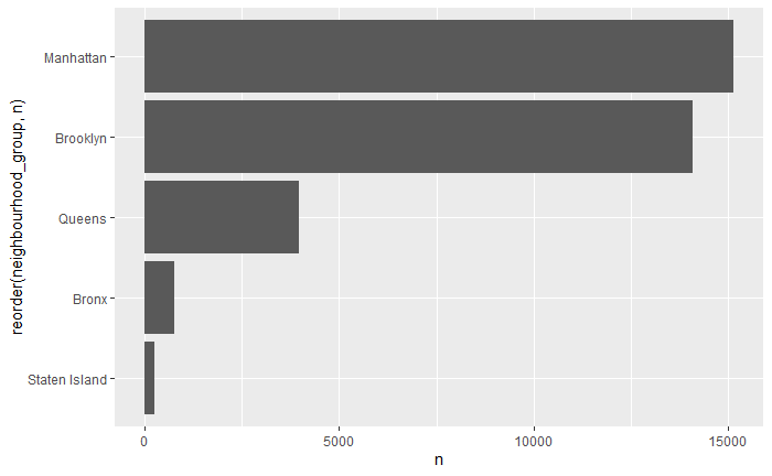
When I looked at the structure of the data from there was also neighbourhood group so I thought it was worth a quick scene to see what that was

neigh <- air_train %>% group_by(neighbourhood_group) %>%
                              summarise(n = n()) %>%
                                  arrange(desc(n))


ggplot(neigh, aes(x = reorder(neighbourhood_group,n), y = n)) + geom_col() + coord_flip()

ggplot(air_train, aes(x = price)) + geom_histogram(binwidth = 10)

Clearly its highly skewed and there are a number of properties apparently $0 per night and a few above $2500 per night. I don’t like log transforming the data because of the impact on interpretability. Maybe in this case it was justified.

10 Min

So now I’m starting to get into the nitty gritty how can i predict the prices better. The frist thing I wanted to look at is the number of properties in a neighbourhood compared to the mean price.

neigh <- air_train %>% group_by(neighbourhood) %>%
summarise(n = n(), medp = mean(price)) %>%
arrange(desc(n))

ggplot(neigh, aes(x = n, y = medp, label= neighbourhood)) + geom_text()

Probably not a very interesting or useful plot but kind of does highlight places like Harlem and Williamsburg are generally cheaper then midtown for example. This looking like a feature to use in the model.

15 min

When looking at the data set I noticed that within the names of the listings there was information on the contents of the listing ( No. Bedrooms and Bathrooms).

names <- air_train %>% select(id, name) %>%
                          separate(name, into = c("s1", "s2", "s3", "s4", "s5", "s6", "s7", "s8", "s9",
                                                  "s10"), sep = " ")  %>%
                            pivot_longer(cols = 2:11, names_to = "s1", values_to = "desc")



names_group <- names %>% filter(!is.na(desc)) %>%
                          group_by(desc) %>%
                              summarise(n = n())

This is the code I used to split the name up I then had a quick scan in the console for top used words

In the most common word obviously people pointing to the location the place is. I didn’t do this but would have been good to look at what words most associated with higher prices. Maybe that could be a feature if that word is in the title or not

names_bed <- names %>% filter(desc %in% c("1br", "2br", "3br", "4br", "1", "2", "3", "4")) %>%
                            mutate(bedrooms = if_else(desc == "1br", "1", 
                                                      if_else(desc == "2br", "2",
                                                        if_else(desc == "3br", "3", 
                                                          if_else(desc == "4br", "4", 
                                                            if_else(desc == "1", "1", 
                                                                if_else(desc == "2", "2", 
                                                                  if_else(desc == "3", "3", 
                                                                    if_else(desc == "4", "4", "0")))))))))

`

So here im converting all the different ways of describing one bedroom into one way and spoiler alert this was a huge mistake.

21 min

names_bed2 <- names %>% filter(desc %in% c("1br", "2br", "3br", "4br", "1", "2", "3", "4", "one", "two", "three", "four")) %>%
                            mutate(bedrooms = if_else(desc == "1br", "1", 
                                                      if_else(desc == "2br", "2",
                                                        if_else(desc == "3br", "3", 
                                                          if_else(desc == "4br", "4", 
                                                            if_else(desc == "1", "1", 
                                                                if_else(desc == "2", "2", 
                                                                  if_else(desc == "3", "3", 
                                                                    if_else(desc == "4", "4", 
                                                                      if_else(desc == "one", "1", 
                                                      if_else(desc == "two", "2",
                                                        if_else(desc == "three", "3", 
                                                          if_else(desc == "four", "4", "")))))))))))))

This is the first part of the big mistake i noticed. I missed the rittn out names of numbers so had to go back and ad them in

train_desc <- names %>% filter(desc %in% c("private", "Cozy", "Private", "Large", "Modern", "Luxary", "Charming", ))

I then added some positive descriptive words that i thought might have some impact on the price.

35 mins

So now im wanting to look at the impact n number of rooms on the price

ggplot(air_train2, aes(x = beds, y = price)) + geom_jitter(alpha = 0.2)

It was no real impact and there is a lot of unknown data. This should have been a red flag but I ignored it stupidly

45 mins

This part is about checking the impact of the room type

ggplot(air_train2, aes(x = room_type, y = price)) + geom_jitter(alpha = 0.2)

Yes that does have an impact. At this point I’m thinking I need to start looking at a model s im more then 45 mins in and maybe i might want to try a few types of model or new features.

air_train2 <- air_train %>% left_join(names_bed2, by = "id") %>%
filter(price < 5000) %>%
filter(price > 0) %>%
select(-desc, -s1) %>%
mutate(beds = if_else(is.na(bedrooms), "unknown", bedrooms)) %>%
select(id, neighbourhood_group, room_type, price, beds)

```{r}

split <- initial_split(air_train2, prop = 0.8)


training <- training(split)


test <- testing(split)





```

So at this point I have created a data frame with the features I am going to use in the first version of my model. I have also used the Tidymodels package to create my training and testing data.

50 Mins

``{r}



air_folds <- bootstraps(training, strata = price)


 ranger_recipe <-
  recipe(formula =  price ~ ., data = training) 


ranger_spec <-
  rand_forest(mtry = tune(), min_n = tune(), trees = 1000) %>%
  set_mode("regression") %>%
  set_engine("ranger")

ranger_workflow <-
  workflow() %>%
  add_recipe(ranger_recipe) %>%
  add_model(ranger_spec)


set.seed(8577)


doParallel::registerDoParallel()
ranger_tune <-
  tune_grid(ranger_workflow,
    resamples = air_folds,
    grid = 10
  )



autoplot(ranger_tune)

So this is where I started to struggle. The training time for this model was extreme and in a time limited competition training a model is dead space. Therefore it needs to be kept down to a minimum. So the output can be understood and directions for improvement can be explored. This train took half an hour as I was trying to tune the model as well.

show_best(ranger_tune, metric = "rmse")

I found my best model parameters but the time was up. In essence I failed and didn’t manage to get a submission within the 2 hours. I still submitted just to get an idea where I finished

Its the private score which counts and that would have had me finishing around 26th. This is in bottom 50% which I would have liked to be in the top 50%. Guess I need to do some more practice in the background and have another go and see where I end up.